How to Read Wall Street Journal Articles
We know that the NY Times data visualizations are pretty awesome, but the Wall Street Periodical's data visualizations are nothing to express joy at. In fact, one of my favorite books on information visualization is by Dona Wong, the former graphics editor of Wall Street Journal and a educatee of Ed Tufte at Yale (and yes, she was at the NY Times too).
The Wall Street Periodical Information Visualization
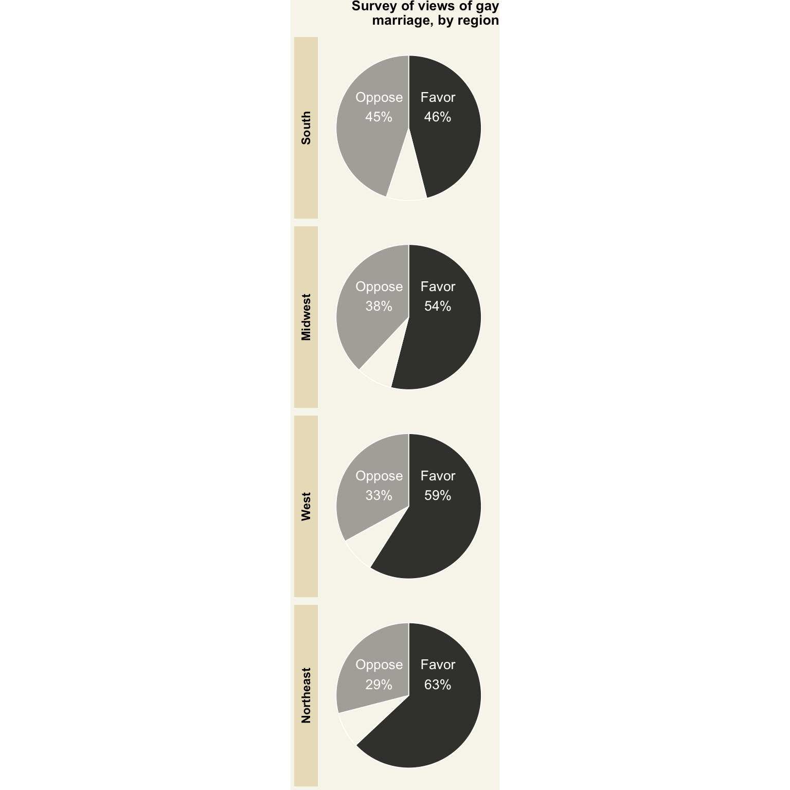
One of my favorite data visualizations from the WSJ is the graphic on Chick-fil-A and the public opinion on same-sexual practice marriage. The WSJ published this graphic in an article after the Chick-fil-A president commented against same-sex activity marriage. The author of this article suggested that Chick-fil-A could afford to express such sentiments because their stores, hence customers, were in regions with bulk of the public'due south opinion was confronting same-sex spousal relationship.

What I liked about the data visualization:
- The graphic itself was very neutral in its color palette and in its conclusions. It left information technology up to the readers to draw whatsoever conclusions.
- The store counts in each state were easy to meet and compare. There was no beautiful icon for each store.
- It removed all the distractions from the data visualization. No extraneous colors, no 3-d effects, no unnecessary information.
- The colors of diverse regions were matched past the colors of the legends for the pie charts.
- Yes, pie charts:
- They were suitable to explicate the three opinion categories.
- They all started with "Favor" at 12 o'clock.
- They were not exploding or were in iii-D, nor did they have l tiny slices.
- The legends were printed only one time.
- A reader could quickly distinguish the public opinion slices using the simple colors.
WSJ Data Visualization in R
Like my previous mail service on NYT's information visualization, I wanted to recreate this WSJ data visualization using R. Here's how I tried to replicate that graphic:
Load favorite libraries
library (rvest) library (stringr) library (dplyr) library (ggplot2) library (scales) library (ggmap) library (readr) library (tidyr) library (zipcode) library (maps) library (jsonlite) library ( grid ) library (gridExtra) data (zipcode) ## load zipcode data in your workspace
library(rvest) library(stringr) library(dplyr) library(ggplot2) library(scales) library(ggmap) library(readr) library(tidyr) library(zipcode) library(maps) library(jsonlite) library(grid) library(gridExtra) data(zipcode) ## load zipcode information in your workspace
-
rvestto scrape information from the spider web -
stringrfor cord manipulation -
dplyrfor data manipulation -
ggplot2for plotting, duh! -
scalesto generate beautiful axis labels -
ggmapto get and plot the United States map -
readrto read data from CSVs -
tidyrto transform data from long to wide form and vice versa -
zipcodeto clean upwardly zipcodes and become the coordinates for each zipcode -
jsonliteto get data from a json object -
gridto line up charts -
gridExtraconsidering stackoverflow said so 🙂
Get Chick-fil-A locations
I plant out that Chick-fil-A listed all its store locations on this page past each country. Every state has a separate page with store locations from that state.
And so, showtime, I got all the states with a shop in an XML document:
states <- read_html( "https://world wide web.Chick-fil-A.com/Locations/Scan" )
states <- read_html("https://www.Chick-fil-A.com/Locations/Scan")
Then, using the CSS selector values, I parsed the XML to extract all the hyperlink text with the URL to each state:
locations <- states %>% html_nodes( "commodity ul li a" ) %>% html_attr( "href" )
locations <- states %>% html_nodes("article ul li a") %>% html_attr("href")
You can utilize Selector Gadget to find CSS selectors of objects on a given web-page. Delight do read rvest'southward documentation for more information on using rvest for web-scraping.
You lot will become a character vector of all the relative urls of each state. Like this:
## [1] "/Locations/Browse/AL" "/Locations/Browse/AZ" "/Locations/Browse/AR" And then, nosotros demand to bring together this relative URL to the acme domain:
locations <- paste0( "https://www.Chick-fil-A.com", locations)
locations <- paste0("https://world wide web.Chick-fil-A.com", locations)
At present, nosotros need to scrape every state page and extract the zipcode of all the stores on that page. I wrote a function to help usa with that:
extract_location <- function ( url ) { read_html( url ) %>% html_nodes( ".location p" ) %>% html_text( ) %>% str_extract( "\\d{5}(?=\northward)" ) }
extract_location <- function(url){ read_html(url) %>% html_nodes(".location p") %>% html_text() %>% str_extract("\\d{5}(?=\n)") }
The function will download each URL, find the div with the location class, convert the lucifer to text, and lastly extract the five digit number (zipcode) using regular expression.
We need to laissez passer the URL of each state to this function. We can achieve that by using sapply role, but be patient as this will accept a minute or two:
locationzips <- sapply (locations, extract_location, Use.NAMES = FALSE)
locationzips <- sapply(locations, extract_location, Apply.NAMES = False)
Clean upwardly the store zip
To make the to a higher place data usable for this data visualization, nosotros need to put the zipcode list in a data frame.
locationzips_df <- data.frame (zips = unlist (locationzips), stringsAsFactors = FALSE)
locationzips_df <- information.frame(zips = unlist(locationzips), stringsAsFactors = FALSE)
If this postal service goes viral, I wouldn't want millions of people trying to download this information from Chick-fil-A's site. I saved you these steps and stored the zips in a csv on my dropbox (find the raw=i parameter at the end to get the file direct and not the preview from dropbox):
locationzips_df <- read_csv( "https://www.dropbox.com/s/x8xwdx61go07e4e/chickfilalocationzips.csv?raw=ane", col_types = "c" )
locationzips_df <- read_csv("https://www.dropbox.com/s/x8xwdx61go07e4e/chickfilalocationzips.csv?raw=i", col_types = "c")
In example nosotros got some bad data, clean up the zipcodes using clean.zipcodes function from the zipcode package.
locationzips_df$zips <- make clean.zipcodes (locationzips_df$zips)
locationzips_df$zips <- make clean.zipcodes(locationzips_df$zips)
Merge coordinate data
Next, we demand to get the coordinate data on each zipcode. Again, the dataset from the zipcode package provides us with that data.
locationzips_df <- merge (locationzips_df, select(zipcode, zip, latitude, longitude, state), by.x = 'zips', past.y = 'aught', all.ten = True)
locationzips_df <- merge(locationzips_df, select(zipcode, zip, latitude, longitude, state), by.x = 'zips', by.y = 'zip', all.x = TRUE)
Calculate the total number of stores by country
This is really easy with some dplyr magic:
rest_cnt_by_state <- count(locationzips_df, country)
rest_cnt_by_state <- count(locationzips_df, state)
This information frame will look something like this:
## # A tibble: 6 × 2 ## country n ## ## 1 AL 77 ## 2 AR 32 ## three AZ 35 ## 4 CA 90 ## five CO 47 ## half dozen CT seven Gather the public stance data
The PRRI portal shows various survey data on American values. The latest year with data is 2015. I dug into the HTML to detect the path to save the JSON data:
region_opinion_favor <- fromJSON( "http://ava.prri.org/ajx_map.regionsdata?category=lgbt_ssm&sc=ii&year=2015&topic=lgbt" )$regions region_opinion_oppose <- fromJSON( "http://ava.prri.org/ajx_map.regionsdata?category=lgbt_ssm&sc=3&yr=2015&topic=lgbt" )$regions
region_opinion_favor <- fromJSON("http://ava.prri.org/ajx_map.regionsdata?category=lgbt_ssm&sc=ii&twelvemonth=2015&topic=lgbt")$regions region_opinion_oppose <- fromJSON("http://ava.prri.org/ajx_map.regionsdata?category=lgbt_ssm&sc=3&year=2015&topic=lgbt")$regions
Adjacent, I added a field to note the opinion:
region_opinion_favor$opi <- 'favor' region_opinion_oppose$opi <- 'oppose'
region_opinion_favor$opi <- 'favor' region_opinion_oppose$opi <- 'oppose'
And then, I manipulated this data to make information technology usable for the pie charts:
region_opinion <- bind_rows(region_opinion_favor, region_opinion_oppose) %>% filter (region != 'national' ) %>% mutate(region = recode(region, "i" = "Northeast", "2" = "Midwest", "3" = "Due south", "four" = "W" ) ) %>% spread(key = opi, value = percent) %>% mutate(other = 100 - favor - oppose) %>% assemble(key = opi, value = percent, -region, - sort ) %>% select( - sort ) %>% mutate(opi = factor (opi, levels = c ( 'oppose', 'other', 'favor' ), ordered = True) )
region_opinion <- bind_rows(region_opinion_favor, region_opinion_oppose) %>% filter(region != 'national') %>% mutate(region = recode(region, "1" = "Northeast", "ii" = "Midwest", "3" = "Southward", "iv" = "West")) %>% spread(key = opi, value = per centum) %>% mutate(other = 100 - favor - oppose) %>% gather(cardinal = opi, value = percent, -region, -sort) %>% select(-sort) %>% mutate(opi = cistron(opi, levels = c('oppose', 'other', 'favor'), ordered = TRUE))
There's a lot of stuff going on in this code. Let me explicate:
- Nosotros bind the two data frames we created
- We remove the data row for the national average
- We recode the numerical regions to text regions
- Nosotros spread the information from long format to wide format. Read tidyr documentation for farther explanation.
- Now that the opinions are two columns, we create some other cavalcade for the remaining/unknown opinions.
- Nosotros bring everything dorsum to long form using
gather. - We remove the
sortcolumn. - We create an
ordered factorfor the opinion. This is so that the oppose stance shows up at the top on the charts.
Afterward all that, nosotros get a data frame that looks like this:
## region opi percent ## 1 Northeast favor 63 ## 2 Midwest favor 54 ## three South favor 46 ## 4 Due west favor 59 ## v Northeast oppose 29 ## 6 Midwest oppose 38 The WSJ data visualization did one more than useful thing: it ordered the pie charts with the regions with most opposition to aforementioned-sex activity marriage at the tiptop. The way to handle this kind of stuff in ggplot is to order the underlying factors.
regions_oppose_sorted <- arrange( filter (region_opinion, opi == 'oppose' ), desc(percent) )$region region_opinion <- mutate(region_opinion, region = factor (region, levels = regions_oppose_sorted, ordered = TRUE) )
regions_oppose_sorted <- arrange(filter(region_opinion, opi == 'oppose'), desc(per centum))$region region_opinion <- mutate(region_opinion, region = factor(region, levels = regions_oppose_sorted, ordered = True))
Now that our dataframe is fix, we tin create the pie charts using ggplot.
Create the pie charts
To create the pie charts in ggplot, nosotros actually create stacked bar graphs first and so change the polar coordinates. We could also utilise the base R plotting functions, but I wanted to test the limits of ggplot.
opin_pie_charts <- ggplot(region_opinion, aes(10 = one, y = percent, make full = opi) ) + geom_bar(width = one,stat = "identity", size = 0.iii, color = "white", alpha = 0.85, evidence.legend = Faux)
opin_pie_charts <- ggplot(region_opinion, aes(10 = one, y = percent, fill = opi)) + geom_bar(width = 1,stat = "identity", size = 0.iii, color = "white", blastoff = 0.85, show.fable = False)
At that place are few things worth explaining here:
- We set up the
aes 10value to 1 equally we really don't accept an x-axis. - We set the
aes fillvalue to the variableopithat has values of oppose, favor and other. - We set the bar
widthto i. I chose this value after some iterations. - Nosotros set the
stattoidentityconsidering nosotros don'tggplotto summate the bar proportions. - Nosotros set the
colorto white – this is the color of the separator between each stack of the bars. - We set the
sizeto 0.3 that gives us reasonable spacing between the stacks. I did so to match the WSJ visualization.
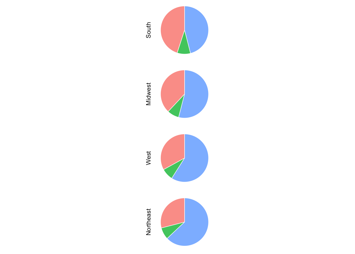
This is the chart we get:

And, your reaction totally may be like this:

first fourth dimension y'all meet the default ggplot stacked bar colors
Well, relax, Kevin. This will get better. I hope.
Adjacent, nosotros add facets to create a separate chart for each region as well as adding the polar coordinates to create the pie chart. I as well added theme_void to remove all the gridlines, centrality lines, and labels.
opin_pie_charts <- opin_pie_charts + facet_grid(region ~ ., switch = "y" ) + coord_polar( "y" ) + theme_void( )
opin_pie_charts <- opin_pie_charts + facet_grid(region ~ ., switch = "y") + coord_polar("y") + theme_void()
Resulting in this:
Feeling better, Kevin?

Let's change the colors, which I found using prototype color picker, of the slices to match with the WSJ's data visualization:
opin_pie_charts <- opin_pie_charts + scale_fill_manual(values = c ( "favor" = "black", "oppose" = "#908E89", "other" = "#F7F3E8" ) )
opin_pie_charts <- opin_pie_charts + scale_fill_manual(values = c("favor" = "black", "oppose" = "#908E89", "other" = "#F7F3E8"))
Giving us this:

Next, add together information tables. I simply picked some good values where it would make sense to evidence the labels:
#add together labels opin_pie_charts <- opin_pie_charts + geom_text(color = "white", size = rel( 3.5 ), aes(x = 1, y = ifelse (opi == 'favor', 15, 85 ), label = ifelse (opi == 'other', NA, paste0(str_to_title(opi), "\due north", percent(per centum/ 100 ) ) ) ) )
#add together labels opin_pie_charts <- opin_pie_charts + geom_text(colour = "white", size = rel(3.five), aes(x = 1, y = ifelse(opi == 'favor', 15, 85), label = ifelse(opi == 'other', NA, paste0(str_to_title(opi), "\due north", percentage(percent/100)))))
Resulting in this:

Side by side, calculation the plot championship as given in the WSJ data visualization:
opin_pie_charts <- opin_pie_charts + ggtitle(label = "Survey of views of gay\northmarriage, by region" ) + theme(plot.championship = element_text(size = 10, confront = "bold", hjust = one ) )
opin_pie_charts <- opin_pie_charts + ggtitle(characterization = "Survey of views of gay\nmarriage, past region") + theme(plot.championship = element_text(size = 10, face = "bold", hjust = 1))

And, the last step:
- change the background color of the region labels,
- emphasize the region labels
- change the console color as well as the plot background color
opin_pie_charts <- opin_pie_charts + theme(strip.background = element_rect(fill = "#E6D9B7" ), strip.text = element_text(face up = "assuming" ), plot.background = element_rect(fill = "#F6F4E8", color = NA), panel.background = element_rect(fill = "#F6F4E8", colour = NA) )
opin_pie_charts <- opin_pie_charts + theme(strip.groundwork = element_rect(fill = "#E6D9B7"), strip.text = element_text(face = "bold"), plot.background = element_rect(fill = "#F6F4E8", colour = NA), panel.background = element_rect(fill up = "#F6F4E8", colour = NA))
Getting us actually close to the WSJ pie charts:
I should say that a pie nautical chart in ggplot is difficult to customize considering you lose one axis. Next fourth dimension, I would try the base R pie chart.
Creating the map
Phew! That was some work to make the pie charts look similar to the WSJ information visualization. At present, more fun: the maps.
First, permit'south become some data ready.
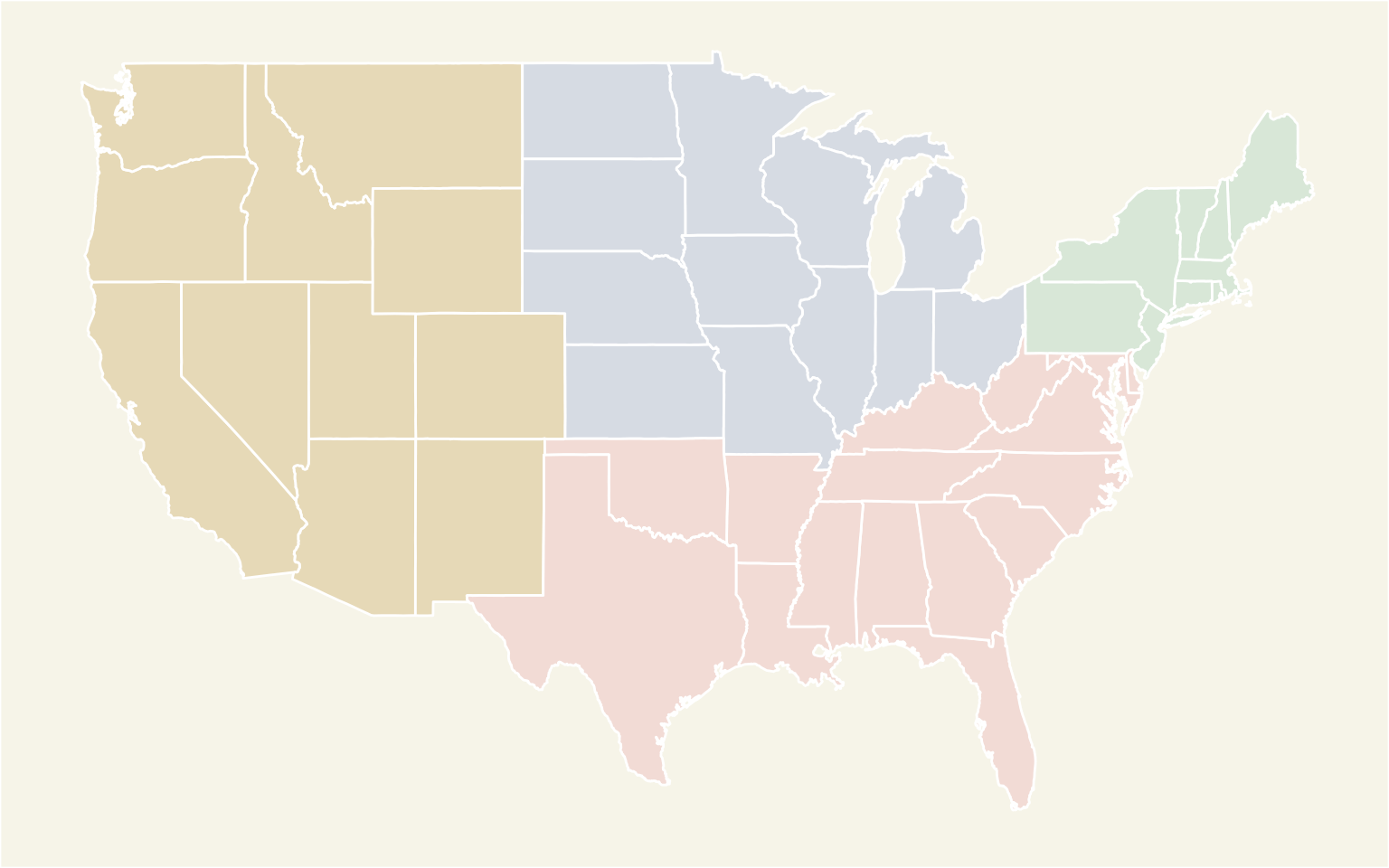
R comes with various data points on each of u.s.. Then, nosotros will become the centers of u.s., abbreviations, regions, and state names.
state_centers_abb <- data.frame (state = tolower ( state.name ), stateabr = state.abb , center_long = state.center $x, center_lat = country.center $y, region = state.region )
state_centers_abb <- information.frame(state = tolower(state.proper name), stateabr = state.abb, center_long = state.center$ten, center_lat = state.center$y, region = land.region)
Which gives united states of america this:
## country stateabr center_long center_lat region ## 1 alabama AL -86.7509 32.5901 South ## 2 alaska AK -127.2500 49.2500 Due west ## three arizona AZ -111.6250 34.2192 West ## 4 arkansas AR -92.2992 34.7336 South ## 5 california CA -119.7730 36.5341 Due west ## half dozen colorado CO -105.5130 38.6777 West The regions in this data prepare have a value of Northward Fundamental; allow's change that to Midwest.
state_centers_abb <- mutate(state_centers_abb, region = recode(region, "North Fundamental" = "Midwest" ) )
state_centers_abb <- mutate(state_centers_abb, region = recode(region, "Northward Cardinal" = "Midwest"))
Next, allow's go the polygon data on each country and merge it with the state centers data frame:
us_map <- map_data( "state" ) us_map <- rename(us_map, state = region) us_map <- inner_join(us_map, state_centers_abb, past = c ( "state" = "state" ) ) us_map <- us_map[ social club (us_map$order), ]
us_map <- map_data("state") us_map <- rename(us_map, state = region) us_map <- inner_join(us_map, state_centers_abb, by = c("state" = "state")) us_map <- us_map[order(us_map$order), ]
While plotting the polygon data using ggplot, you take to make sure that the order column of the polygon data frame is ordered, otherwise, you volition get some wacky looking shapes.
With some prep work done, let the fun begin. Let's create the base map:
base_plot <- ggplot( data = left_join(us_map, rest_cnt_by_state, by = c ( "stateabr" = "state" ) ), aes(x = long, y = lat, group = group, order = society, fill up = region) ) + geom_polygon(color = "white" )
base_plot <- ggplot(information = left_join(us_map, rest_cnt_by_state, by = c("stateabr" = "land")), aes(ten = long, y = lat, grouping = grouping, order = order, fill = region)) + geom_polygon(colour = "white")
You will note that I've joined the polygon data frame with the counts of restaurants in each land. Also, similar to the stacked bar graphs, I've separated each country with the white color, giving us this:

I already see Kevin going crazy!
I again used the epitome color picker to select the colors from the WSJ data visualization and assigned them manually to each region. I likewise removed the legend:
base_plot <- base_plot + scale_fill_manual(values = c ( "West" = "#E6D9B7", "South" = "#F2DBD5", "Northeast" = "#D8E7D7", "Midwest" = "#D6DBE3" ), guide = Simulated)
base_plot <- base_plot + scale_fill_manual(values = c("West" = "#E6D9B7", "South" = "#F2DBD5", "Northeast" = "#D8E7D7", "Midwest" = "#D6DBE3"), guide = FALSE)
Generating this:

Next, remove all the distractions and modify the background color:
base_plot <- base_plot + theme(axis.championship = element_blank( ), axis.ticks = element_blank( ), axis.line = element_blank( ), axis.text = element_blank( ), panel.grid = element_blank( ), console.border = element_blank( ), plot.background = element_rect(fill = "#F6F4E8" ), panel.background = element_rect(fill up = "#F6F4E8" ) )
base_plot <- base_plot + theme(axis.title = element_blank(), axis.ticks = element_blank(), axis.line = element_blank(), axis.text = element_blank(), panel.grid = element_blank(), panel.border = element_blank(), plot.background = element_rect(fill up = "#F6F4E8"), panel.groundwork = element_rect(fill = "#F6F4E8"))
Giving us this:
Side by side upwards is adding the circles for restaurant counts.
base_plot <- base_plot + geom_point(aes(size = n, x = center_long, y = center_lat), shape = ane, stroke = 0.5, colour = "grey60", inherit.aes = FALSE) + scale_size_area(max_size = 18, breaks = c ( 0, 10, 100, 300 ), guide = FALSE) + scale_shape(solid = False)
base_plot <- base_plot + geom_point(aes(size = northward, x = center_long, y = center_lat), shape = 1, stroke = 0.5, color = "grey60", inherit.aes = Faux) + scale_size_area(max_size = 18, breaks = c(0, x, 100, 300), guide = False) + scale_shape(solid = FALSE)
OK. In that location is a lot of stuff going on hither. First, we employ geom_point to create the circles at the center of each state. The size of the circle is dictated past the number of restaurants in each state. The stroke parameters controls the thickness of the circle. Nosotros besides are using inherit.aes = FALSE to create new aesthetics for this geom.
The scale_size_area is very of import considering as the documentation says:
scale_size scales area, scale_radius scales radius. The size aesthetic is nigh unremarkably used for points and text, and humans perceive the surface area of points (non their radius), and so this provides for optimal perception. scale_size_area ensures that a value of 0 is mapped to a size of 0.
Don't allow this happen to you! Employ the area and non the radius.
I as well increased the size of the circles and gave breaks manually to the circle sizes.
Generating this:

Since we removed the legend for the circumvolve size and the WSJ graphic had one, allow's endeavour to add together that back in. This was challenging and hardly accurate. I played with some sizes and eyeballed to match the radii of different circles. I don't recommend this at all. This is better handled in postal service-processing using Inkscape or Illustrator.
Please add the circles every bit a legend in post-processing. Adding circumvolve grobs is not authentic and doesn't produce the desired results.
base_plot <- base_plot + annotation_custom(grob = circleGrob(r = unit of measurement( i.4, "lines" ), gp = gpar(fill = "gray87", alpha = 0.5 ) ), xmin = - 79, xmax = - 77, ymin = 48 , ymax = 49 ) + annotation_custom(grob = circleGrob(r = unit( 0.7, "lines" ), gp = gpar(make full = "gray85", alpha = 0.87 ) ), xmin = - 79, xmax = - 77, ymin = 47.4, ymax = 48 ) + annotation_custom(grob = circleGrob(r = unit( 0.3, "lines" ), gp = gpar(fill = "gray80", alpha = 0.95 ) ), xmin = - 79, xmax = - 77, ymin = 46.5, ymax = 48 )
base_plot <- base_plot + annotation_custom(grob = circleGrob(r = unit of measurement(1.4, "lines"), gp = gpar(fill = "gray87", blastoff = 0.5)), xmin = -79, xmax = -77, ymin = 48 , ymax = 49) + annotation_custom(grob = circleGrob(r = unit of measurement(0.7, "lines"), gp = gpar(fill = "gray85", blastoff = 0.87)), xmin = -79, xmax = -77, ymin = 47.4, ymax = 48) + annotation_custom(grob = circleGrob(r = unit(0.3, "lines"), gp = gpar(fill = "gray80", alpha = 0.95)), xmin = -79, xmax = -77, ymin = 46.five, ymax = 48)
Giving united states of america:

Let'south add the title:
base_plot <- base_plot + ggtitle(label = "Number of Chick-fil-A resturants by state and region" ) + theme(plot.title = element_text(size = 10, face = "bold", hjust = 0.fourteen, vjust = - 5 ) )
base_plot <- base_plot + ggtitle(label = "Number of Chick-fil-A resturants by state and region") + theme(plot.title = element_text(size = 10, confront = "bold", hjust = 0.14, vjust = -5))
Merging united states and pie charts
This is the easiest step of all. We use the grid.adapt function to merge the two plots to create our own WSJ information visualization in R.
png ( "wsj-Chick-fil-A-data-visualization-r-plot.png", width = 800, top = 500, units = "px" ) grid.suit (base_plot, opin_pie_charts, widths= c ( 4, 1 ), nrow = 1 ) dev.off ( )
png("wsj-Chick-fil-A-data-visualization-r-plot.png", width = 800, height = 500, units = "px") grid.adapt(base_plot, opin_pie_charts, widths= c(4, 1), nrow = 1) dev.off()
Here it is:
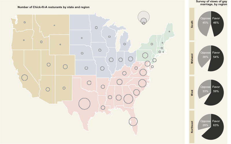
What do yous call back?
Some things I couldn't brand work:
- Alter the colour of the facet of the pie charts. I toyed with
strip.textsettings, but I couldn't change all the colors. Possibly, it is easy to do so in thebase Rpie charts. - The circumvolve-in-circle legend. I got the circles, but not the numbers.
- The 'other' category label in the pie chart.
- Brand the circles on the maps look less jagged-y.
Does the data visualization still work?
Of course, the public opinion over same-sex matrimony has changed across usa and Chick-fil-A has opened up more stores across the country.
It however does wait similar that bigger circles are in the regions where people oppose the same-sex marriage.
I wanted to question that. According to the Pew research center information, only 33% of Republicans favor same-sex matrimony. And then, if we were to plot the 2016 U.S. Presidential elections past county and plot each zipcode of Chick-fil-A stores, nosotros tin can see whether there are more stores in counties voting for Donald Trump.
Permit's become started so.
Go the county level information. Tony McGovern already did all the hard work:
cnty_results <- read_csv( "https://raw.githubusercontent.com/tonmcg/County_Level_Election_Results_12-16/master/2016_US_County_Level_Presidential_Results.csv" ) cnty_results <- mutate(cnty_results, per_point_diff = per_gop - per_dem, county_name = tolower (str_replace(county_name, " County", "" ) ), county_name = tolower (str_replace(county_name, " parish", "" ) ) )
cnty_results <- read_csv("https://raw.githubusercontent.com/tonmcg/County_Level_Election_Results_12-16/master/2016_US_County_Level_Presidential_Results.csv") cnty_results <- mutate(cnty_results, per_point_diff = per_gop - per_dem, county_name = tolower(str_replace(county_name, " County", "")), county_name = tolower(str_replace(county_name, " parish", "")))
Become the canton map polygon data:
county_map <- map_data( "canton" ) county_map <- rename(county_map, state = region, county = subregion) county_map$stateabr <- land.abb [ match (county_map$state, tolower ( state.proper name ) ) ]
county_map <- map_data("canton") county_map <- rename(county_map, state = region, county = subregion) county_map$stateabr <- state.abb[match(county_map$state, tolower(state.name))]
Join the polygon with county results:
cnty_map_results <- left_join(county_map, cnty_results, by = c ( "stateabr" = "state_abbr", "county" = "county_name" ) ) %>% accommodate( guild, group)
cnty_map_results <- left_join(county_map, cnty_results, by = c("stateabr" = "state_abbr", "county" = "county_name")) %>% adapt(order, group)
Plot the results and counties:
cnty_plot <- ggplot( data = cnty_map_results, aes(x = long, y = lat, grouping = group, order = society ) ) + geom_polygon(aes(fill up = per_point_diff), colour = "gray90", size = 0.1 )
cnty_plot <- ggplot(data = cnty_map_results, aes(x = long, y = lat, group = grouping, order = order)) + geom_polygon(aes(fill = per_point_diff), color = "gray90", size = 0.1)
This what we become:

Now, we fill up the map with red and blue colors for the republican and democratic voting counties:
cnty_plot <- cnty_plot + scale_fill_gradient2(midpoint = 0, low = "#2062A1", mid = "white", high = "ruddy", na.value = "white", breaks = seq (from = 0, to = ane, length.out = vii ), guide = FALSE)
cnty_plot <- cnty_plot + scale_fill_gradient2(midpoint = 0, low = "#2062A1", mid = "white", high = "red", na.value = "white", breaks = seq(from = 0, to = ane, length.out = seven), guide = FALSE)
Generating this:

Permit'south remove all the distractions and add the store locations past zipcode:
cnty_plot <- cnty_plot + theme_void( ) + geom_point( data = locationzips_df, aes(x = longitude, y = latitude), size = 0.3, alpha = 0.2, inherit.aes = FALSE)
cnty_plot <- cnty_plot + theme_void() + geom_point(information = locationzips_df, aes(x = longitude, y = latitude), size = 0.iii, alpha = 0.2, inherit.aes = Imitation)
Giving u.s.a. this:
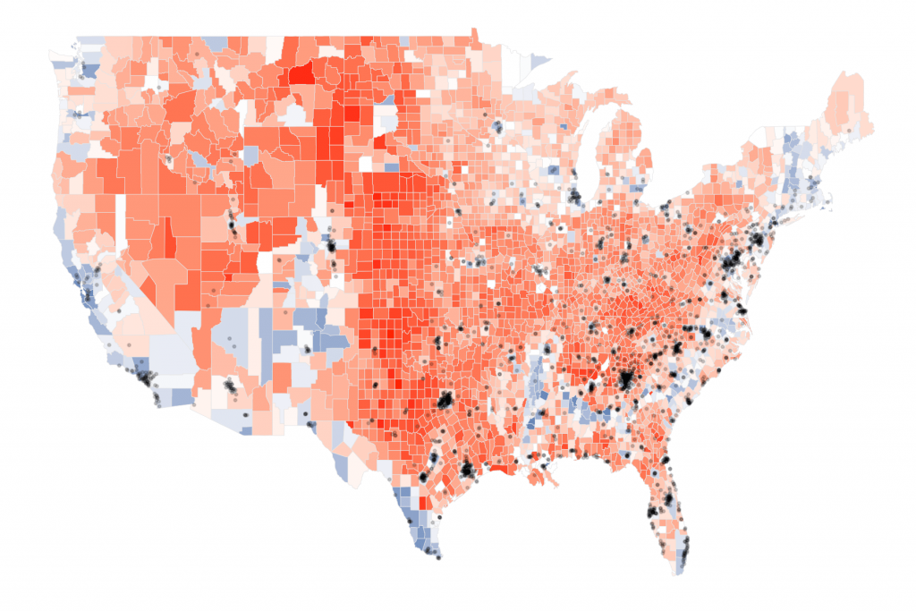
Very dissimilar picture, wouldn't you say? It actually looks similar that the store locations are present in more than autonomous leaning counties or at least the counties that are as divided betwixt the republican and democratic votes.
Of course, it is possible that I messed something upwardly. Simply, I tin can conclude two things based on this chart:
- Aggregation can mislead us to come across the non-existent patterns
- A person's political identification or views has nothing to do with the nutrient he or she likes. And, the Chick-fil-A leaders know that.
What exercise you lot think?
Consummate Script
library (rvest) library (stringr) library (dplyr) library (ggplot2) library (scales) library (ggmap) library (readr) library (tidyr) library (zipcode) library (maps) library (jsonlite) library ( grid ) library (gridExtra) data (zipcode) ## load zipcode data in your workspace states <- read_html( "https://world wide web.Chick-fil-A.com/Locations/Browse" ) locations <- states %>% html_nodes( "article ul li a" ) %>% html_attr( "href" ) locations <- paste0( "https://www.Chick-fil-A.com", locations) extract_location <- function ( url ) { read_html( url ) %>% html_nodes( ".location p" ) %>% html_text( ) %>% str_extract( "\\d{v}(?=\n)" ) } locationzips <- sapply (locations, extract_location, Use.NAMES = Simulated) locationzips_df <- data.frame (zips = unlist (locationzips), stringsAsFactors = Fake) #locationzips_df <- read_csv("https://www.dropbox.com/s/x8xwdx61go07e4e/chickfilalocationzips.csv?raw=1", col_types = "c") locationzips_df$zips <- clean.zipcodes (locationzips_df$zips) locationzips_df <- merge (locationzips_df, select(zipcode, zip, latitude, longitude, state), by.x = 'zips', by.y = 'zip', all.ten = TRUE) est_cnt_by_state <- count(locationzips_df, state) head (rest_cnt_by_state) region_opinion_favor <- fromJSON( "http://ava.prri.org/ajx_map.regionsdata?category=lgbt_ssm&sc=2&year=2015&topic=lgbt" )$regions region_opinion_oppose <- fromJSON( "http://ava.prri.org/ajx_map.regionsdata?category=lgbt_ssm&sc=3&year=2015&topic=lgbt" )$regions region_opinion_favor$opi <- 'favor' region_opinion_oppose$opi <- 'oppose' region_opinion <- bind_rows(region_opinion_favor, region_opinion_oppose) %>% filter (region != 'national' ) %>% mutate(region = recode(region, "one" = "Northeast", "ii" = "Midwest", "3" = "Due south", "4" = "West" ) ) %>% spread(key = opi, value = percent) %>% mutate(other = 100 - favor - oppose) %>% gather(key = opi, value = percentage, -region, - sort ) %>% select( - sort ) %>% mutate(opi = factor (opi, levels = c ( 'oppose', 'other', 'favor' ), ordered = TRUE) ) head (region_opinion) regions_oppose_sorted <- suit( filter (region_opinion, opi == 'oppose' ), desc(percent) )$region region_opinion <- mutate(region_opinion, region = cistron (region, levels = regions_oppose_sorted, ordered = TRUE) ) opin_pie_charts <- ggplot(region_opinion, aes(x = 1, y = percent, fill up = opi) ) + geom_bar(width = i,stat = "identity", size = 0.iii, color = "white", alpha = 0.85, show.legend = FALSE) plot (opin_pie_charts) opin_pie_charts <- opin_pie_charts + facet_grid(region ~ ., switch = "y" ) + coord_polar( "y" ) + theme_void( ) plot (opin_pie_charts) opin_pie_charts <- opin_pie_charts + scale_fill_manual(values = c ( "favor" = "blackness", "oppose" = "#908E89", "other" = "#F7F3E8" ) ) plot (opin_pie_charts) #add labels opin_pie_charts <- opin_pie_charts + geom_text(colour = "white", size = rel( 3.v ), aes(ten = 1, y = ifelse (opi == 'favor', 15, 85 ), label = ifelse (opi == 'other', NA, paste0(str_to_title(opi), "\n", percent(percentage/ 100 ) ) ) ) ) plot (opin_pie_charts) opin_pie_charts <- opin_pie_charts + ggtitle(label = "Survey of views of gay\nmarriage, past region" ) + theme(plot.title = element_text(size = 10, face = "bold", hjust = i ) ) plot (opin_pie_charts) opin_pie_charts <- opin_pie_charts + theme(strip.background = element_rect(fill = "#E6D9B7" ), strip.text = element_text(face up = "bold" ), plot.groundwork = element_rect(fill = "#F6F4E8", color = NA), panel.background = element_rect(fill up = "#F6F4E8", colour = NA) ) plot (opin_pie_charts) state_centers_abb <- data.frame (state = tolower ( state.proper name ), stateabr = state.abb , center_long = country.center $x, center_lat = state.center $y, region = state.region ) head (state_centers_abb) state_centers_abb <- mutate(state_centers_abb, region = recode(region, "N Central" = "Midwest" ) ) us_map <- map_data( "state" ) us_map <- rename(us_map, land = region) us_map <- inner_join(us_map, state_centers_abb, by = c ( "state" = "land" ) ) us_map <- us_map[ lodge (us_map$lodge), ] base_plot <- ggplot( data = left_join(us_map, rest_cnt_by_state, by = c ( "stateabr" = "country" ) ), aes(x = long, y = lat, grouping = group, order = order, fill up = region) ) + geom_polygon(color = "white" ) plot (base_plot) base_plot <- base_plot + scale_fill_manual(values = c ( "West" = "#E6D9B7", "South" = "#F2DBD5", "Northeast" = "#D8E7D7", "Midwest" = "#D6DBE3" ), guide = FALSE) plot (base_plot) base_plot <- base_plot + theme(axis.championship = element_blank( ), axis.ticks = element_blank( ), axis.line = element_blank( ), axis.text = element_blank( ), console.grid = element_blank( ), panel.border = element_blank( ), plot.background = element_rect(fill up = "#F6F4E8" ), panel.background = element_rect(fill = "#F6F4E8" ) ) plot (base_plot) base_plot <- base_plot + geom_point(aes(size = northward, x = center_long, y = center_lat), shape = 1, stroke = 0.5, color = "grey60", inherit.aes = FALSE) + scale_size_area(max_size = xviii, breaks = c ( 0, 10, 100, 300 ), guide = Simulated) + scale_shape(solid = Imitation) plot (base_plot) base_plot <- base_plot + annotation_custom(grob = circleGrob(r = unit of measurement( 1.4, "lines" ), gp = gpar(fill = "gray87", alpha = 0.5 ) ), xmin = - 79, xmax = - 77, ymin = 48 , ymax = 49 ) + annotation_custom(grob = circleGrob(r = unit of measurement( 0.7, "lines" ), gp = gpar(fill = "gray85", alpha = 0.87 ) ), xmin = - 79, xmax = - 77, ymin = 47.four, ymax = 48 ) + annotation_custom(grob = circleGrob(r = unit( 0.iii, "lines" ), gp = gpar(fill = "gray80", alpha = 0.95 ) ), xmin = - 79, xmax = - 77, ymin = 46.5, ymax = 48 ) plot (base_plot) base_plot <- base_plot + ggtitle(label = "Number of Chick-fil-A resturants by state and region" ) + theme(plot.championship = element_text(size = 10, face = "bold", hjust = 0.xiv, vjust = - 5 ) ) png ( "wsj-Chick-fil-A-data-visualization-r-plot.png", width = 800, summit = 500, units = "px" ) filigree.conform (base_plot, opin_pie_charts, widths= c ( 4, 1 ), nrow = 1 ) dev.off ( ) cnty_results <- read_csv( "https://raw.githubusercontent.com/tonmcg/County_Level_Election_Results_12-16/master/2016_US_County_Level_Presidential_Results.csv" ) cnty_results <- mutate(cnty_results, per_point_diff = per_gop - per_dem, county_name = tolower (str_replace(county_name, " County", "" ) ), county_name = tolower (str_replace(county_name, " parish", "" ) ) ) county_map <- map_data( "canton" ) county_map <- rename(county_map, state = region, county = subregion) county_map$stateabr <- state.abb [ lucifer (county_map$state, tolower ( country.name ) ) ] cnty_map_results <- left_join(county_map, cnty_results, by = c ( "stateabr" = "state_abbr", "county" = "county_name" ) ) %>% arrange( order, group) cnty_plot <- ggplot( data = cnty_map_results, aes(x = long, y = lat, grouping = group, order = order ) ) + geom_polygon(aes(fill = per_point_diff), color = "gray90", size = 0.1 ) plot (cnty_plot) cnty_plot <- cnty_plot + scale_fill_gradient2(midpoint = 0, low = "#2062A1", mid = "white", high = "red", na.value = "white", breaks = seq (from = 0, to = i, length.out = 7 ), guide = FALSE) plot (cnty_plot) cnty_plot <- cnty_plot + theme_void( ) + geom_point( data = locationzips_df, aes(10 = longitude, y = breadth), size = 0.3, alpha = 0.2, inherit.aes = FALSE)
library(rvest) library(stringr) library(dplyr) library(ggplot2) library(scales) library(ggmap) library(readr) library(tidyr) library(zipcode) library(maps) library(jsonlite) library(grid) library(gridExtra) information(zipcode) ## load zipcode information in your workspace states <- read_html("https://www.Chick-fil-A.com/Locations/Browse") locations <- states %>% html_nodes("article ul li a") %>% html_attr("href") locations <- paste0("https://www.Chick-fil-A.com", locations) extract_location <- function(url){ read_html(url) %>% html_nodes(".location p") %>% html_text() %>% str_extract("\\d{five}(?=\n)") } locationzips <- sapply(locations, extract_location, Utilise.NAMES = FALSE) locationzips_df <- information.frame(zips = unlist(locationzips), stringsAsFactors = Faux) #locationzips_df <- read_csv("https://world wide web.dropbox.com/due south/x8xwdx61go07e4e/chickfilalocationzips.csv?raw=i", col_types = "c") locationzips_df$zips <- clean.zipcodes(locationzips_df$zips) locationzips_df <- merge(locationzips_df, select(zipcode, zip, latitude, longitude, state), past.x = 'zips', by.y = 'nothing', all.x = Truthful) est_cnt_by_state <- count(locationzips_df, state) head(rest_cnt_by_state) region_opinion_favor <- fromJSON("http://ava.prri.org/ajx_map.regionsdata?category=lgbt_ssm&sc=2&year=2015&topic=lgbt")$regions region_opinion_oppose <- fromJSON("http://ava.prri.org/ajx_map.regionsdata?category=lgbt_ssm&sc=3&year=2015&topic=lgbt")$regions region_opinion_favor$opi <- 'favor' region_opinion_oppose$opi <- 'oppose' region_opinion <- bind_rows(region_opinion_favor, region_opinion_oppose) %>% filter(region != 'national') %>% mutate(region = recode(region, "1" = "Northeast", "2" = "Midwest", "three" = "South", "iv" = "West")) %>% spread(key = opi, value = percent) %>% mutate(other = 100 - favor - oppose) %>% gather(central = opi, value = percent, -region, -sort) %>% select(-sort) %>% mutate(opi = factor(opi, levels = c('oppose', 'other', 'favor'), ordered = TRUE)) head(region_opinion) regions_oppose_sorted <- accommodate(filter(region_opinion, opi == 'oppose'), desc(percent))$region region_opinion <- mutate(region_opinion, region = factor(region, levels = regions_oppose_sorted, ordered = Truthful)) opin_pie_charts <- ggplot(region_opinion, aes(10 = 1, y = pct, make full = opi)) + geom_bar(width = i,stat = "identity", size = 0.iii, color = "white", alpha = 0.85, bear witness.legend = Faux) plot(opin_pie_charts) opin_pie_charts <- opin_pie_charts + facet_grid(region ~ ., switch = "y") + coord_polar("y") + theme_void() plot(opin_pie_charts) opin_pie_charts <- opin_pie_charts + scale_fill_manual(values = c("favor" = "black", "oppose" = "#908E89", "other" = "#F7F3E8")) plot(opin_pie_charts) #add labels opin_pie_charts <- opin_pie_charts + geom_text(color = "white", size = rel(iii.5), aes(ten = 1, y = ifelse(opi == 'favor', 15, 85), characterization = ifelse(opi == 'other', NA, paste0(str_to_title(opi), "\northward", percent(pct/100))))) plot(opin_pie_charts) opin_pie_charts <- opin_pie_charts + ggtitle(label = "Survey of views of gay\nmarriage, by region") + theme(plot.title = element_text(size = 10, face = "assuming", hjust = i)) plot(opin_pie_charts) opin_pie_charts <- opin_pie_charts + theme(strip.background = element_rect(fill = "#E6D9B7"), strip.text = element_text(face = "assuming"), plot.background = element_rect(make full = "#F6F4E8", color = NA), panel.background = element_rect(make full = "#F6F4E8", color = NA)) plot(opin_pie_charts) state_centers_abb <- information.frame(country = tolower(state.name), stateabr = country.abb, center_long = country.center$10, center_lat = state.center$y, region = country.region) caput(state_centers_abb) state_centers_abb <- mutate(state_centers_abb, region = recode(region, "North Central" = "Midwest")) us_map <- map_data("country") us_map <- rename(us_map, state = region) us_map <- inner_join(us_map, state_centers_abb, by = c("state" = "land")) us_map <- us_map[lodge(us_map$club), ] base_plot <- ggplot(data = left_join(us_map, rest_cnt_by_state, past = c("stateabr" = "state")), aes(x = long, y = lat, group = group, society = order, fill = region)) + geom_polygon(color = "white") plot(base_plot) base_plot <- base_plot + scale_fill_manual(values = c("Due west" = "#E6D9B7", "S" = "#F2DBD5", "Northeast" = "#D8E7D7", "Midwest" = "#D6DBE3"), guide = FALSE) plot(base_plot) base_plot <- base_plot + theme(axis.title = element_blank(), axis.ticks = element_blank(), axis.line = element_blank(), centrality.text = element_blank(), panel.grid = element_blank(), panel.border = element_blank(), plot.background = element_rect(fill = "#F6F4E8"), panel.background = element_rect(fill = "#F6F4E8")) plot(base_plot) base_plot <- base_plot + geom_point(aes(size = north, x = center_long, y = center_lat), shape = 1, stroke = 0.5, color = "grey60", inherit.aes = FALSE) + scale_size_area(max_size = 18, breaks = c(0, ten, 100, 300), guide = FALSE) + scale_shape(solid = Simulated) plot(base_plot) base_plot <- base_plot + annotation_custom(grob = circleGrob(r = unit of measurement(1.4, "lines"), gp = gpar(fill = "gray87", blastoff = 0.5)), xmin = -79, xmax = -77, ymin = 48 , ymax = 49) + annotation_custom(grob = circleGrob(r = unit(0.7, "lines"), gp = gpar(fill = "gray85", alpha = 0.87)), xmin = -79, xmax = -77, ymin = 47.4, ymax = 48) + annotation_custom(grob = circleGrob(r = unit(0.3, "lines"), gp = gpar(make full = "gray80", blastoff = 0.95)), xmin = -79, xmax = -77, ymin = 46.5, ymax = 48) plot(base_plot) base_plot <- base_plot + ggtitle(label = "Number of Chick-fil-A resturants by state and region") + theme(plot.title = element_text(size = 10, face up = "bold", hjust = 0.fourteen, vjust = -5)) png("wsj-Chick-fil-A-data-visualization-r-plot.png", width = 800, superlative = 500, units = "px") grid.arrange(base_plot, opin_pie_charts, widths= c(4, 1), nrow = 1) dev.off() cnty_results <- read_csv("https://raw.githubusercontent.com/tonmcg/County_Level_Election_Results_12-xvi/principal/2016_US_County_Level_Presidential_Results.csv") cnty_results <- mutate(cnty_results, per_point_diff = per_gop - per_dem, county_name = tolower(str_replace(county_name, " County", "")), county_name = tolower(str_replace(county_name, " parish", ""))) county_map <- map_data("county") county_map <- rename(county_map, state = region, county = subregion) county_map$stateabr <- state.abb[match(county_map$state, tolower(state.name))] cnty_map_results <- left_join(county_map, cnty_results, past = c("stateabr" = "state_abbr", "county" = "county_name")) %>% arrange(order, group) cnty_plot <- ggplot(data = cnty_map_results, aes(x = long, y = lat, group = group, order = lodge)) + geom_polygon(aes(fill = per_point_diff), color = "gray90", size = 0.one) plot(cnty_plot) cnty_plot <- cnty_plot + scale_fill_gradient2(midpoint = 0, low = "#2062A1", mid = "white", high = "red", na.value = "white", breaks = seq(from = 0, to = 1, length.out = 7), guide = FALSE) plot(cnty_plot) cnty_plot <- cnty_plot + theme_void() + geom_point(data = locationzips_df, aes(x = longitude, y = latitude), size = 0.iii, alpha = 0.2, inherit.aes = FALSE)
About the Author
A co-author of Data Scientific discipline for Fundraising, an accolade winning keynote speaker, Ashutosh R. Nandeshwar is one of the few analytics professionals in the higher education manufacture who has adult analytical solutions for all stages of the student life cycle (from recruitment to giving). He enjoys speaking about the ability of information, besides as ranting about data professionals who hunt after "interesting" things. He earned his PhD/MS from West Virginia University and his BEng from Nagpur University, all in industrial engineering. Currently, he is leading the data science, reporting, and prospect development efforts at the Academy of Southern California.
Source: https://nandeshwar.info/data-visualization/wall-street-journal-data-visualization-r/