Does a Continuous Probability Distribution Have to Approach Zero

We consider distributions that have a continuous range of values. Discrete probability distributions where defined by a probability mass function. Analogously continuous probability distributions are defined by a probability density function.

(This is a section in the notes here.)

Definition [Probability Density Function] A probability density function (pdf) is a function $f: \mathbb R \rightarrow \mathbb R_+$ that has two properties

(Positive) For $x \in \mathbb R$

$f(x) \geq 0.$

(Integrates to one) $\begin{aligned} \int_{-\infty}^\infty f(x) dx = 1 \, . %\end{aligned}$

Screenshot 2021-11-18 at 16.26.40

From this we can define the following.

Definition [Continuous Probability Distribution] A random variable $X$ with values in $\mathbb R$ has a continuous probability distribution with pdf $f(x)$ if $\begin{aligned} F(x) := \mathbb P(X \leq x) = \int_{-\infty}^x f(y)dy \,. %\end{aligned}$

Screenshot 2021-11-18 at 16.27.30

As before, $F(x)$ is called the cumulative distribution function (CDF). As before it satisfies

and also it satisfies $\begin{aligned} \label{e:FTC} F'(x) = f(x) . %\end{aligned}$ $F'(x) = f(x)$

A key observation is that when making the conceptual switch from (discrete) probability mass functions to (continuous) probability density distributions, we have replaced summations with integration. This is the main difference, and since most properties of sums apply to integrals¹ many properties follow over for continuous random variables.

A few observations. Notice that the Equation is a consequence of the Fundamental Theorem of Calculus. Note while a pmf must be bounded above by $1$ , in principle, a pdf can be unbounded.² Notice we may want to restrict a continuous random variable to a range of values. For example, we may want to assume that our random variable is positive, in this case the pdf will satisfy $f(x) = 0$ for $x < 0$ . Notice it does not make sense to think of a continuous random variable as taking any specific value since the integral of a point is zero. Instead we often think of the random variable belonging to some range of values. For instance, for $a<b$ , we have $\begin{aligned} \mathbb P(a < X \leq b) = \mathbb P( X\leq b) - \mathbb P( X \leq a) = F(b) -F(a) = \int_a^b f(x)dx \, . %\end{aligned}$

Screenshot 2021-11-18 at 16.28.24

Joint distributions. We can consider the pdf for two random variables (or more). If $X$ , $Y$ are continuous random variables (defined on the same probability space) then their joint pdf is a function $f(x,y)$ such that

and from this $\begin{aligned} \mathbb P(X \leq a, Y \leq b) = \int_{-\infty}^a \int_{-\infty}^b f(x,y) dx dy \, . \footnote{Recall that when you have a double integral like this you integrate the integral in the middle first with respect to $x$ (treating $y$ as a fixed number) and they you integrate the outside with respect to $y$.} %\end{aligned}$ If $X$ and $Y$ are independent then the joint pdf is the product of the pdfs $\begin{aligned} f(x,y) = f_X(x) f_Y(y) \, . %\end{aligned}$

$f(x,y) = f_X(x) f_Y(y).$

All other the above extends out to more than two random variables $X_1,...,X_n$ in the way you might naturally expect. E.g. the pdf is a function of the form $f(x_1,...,x_n)$ .

Expectations

Analogous to the expectation in discrete random variables we have the following definition.

Definition [Expectation, continuous case] The expectation of a continuous random variable $X$ is given by $\begin{aligned} \mathbb E [ X] := \int_{-\infty}^\infty x f(x) dx \, . %\end{aligned}$

Screenshot 2021-11-18 at 16.29.50

Similarly the variance is defined much as before $\begin{aligned} \mathbb V( X ) = \mathbb E [ (X-\mathbb E[X])^2] = \mathbb E[X^2] - \mathbb E[X]^2 = \int_{-\infty}^\infty x^2 f(x)dx - \left( \int_{-\infty}^\infty x f(x)dx \right)^2. %\end{aligned}$

Screenshot 2021-11-18 at 16.30.09

The following proposition is an amalgamation of the lemmas that we had for discrete random variables.

Screenshot 2021-11-18 at 16.30.38

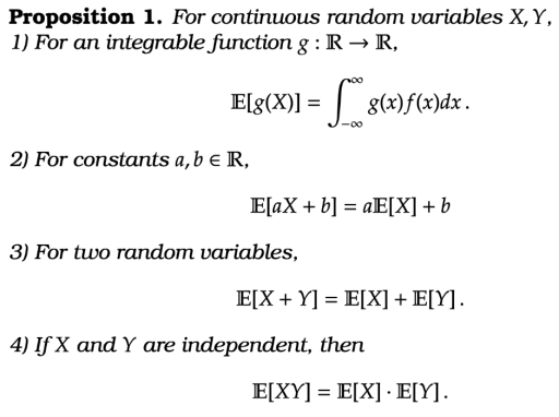
The proof of the above result really follow by an almost identical proof to the earlier discrete results. Just replace the summations with integrals. For that reason we omit the proof of this proposition.

The Normal Distribution

The normal distribution arrises in many situations involving measurement. E.g. the distributions of heights, the relative change in a stock index, the measurement of physical phenomena (e.g. a comet passing the sun), the result from an election poll, the distribution of heat.

The normal distribution is, perhaps, the most important probability distribution. Why is this? Well roughly because it is the distributions that arises when you add up lots of small independent errors. This is more formally states as a result called the central limit theorem, which we will discuss shortly.

Definition [Standard Normal Distribution] The standard normal distribution has probability density function $\phi(x) = \frac{1}{\sqrt{2\pi} } \exp\Big\{-\frac{x^2}{2}\Big\},$ for $-\infty < x < \infty$ . If a random variable $Z$ is a standard normal random variable we write $Z\sim \mathcal N(0,1)$ . The cumulative distribution function is $\begin{aligned} \Phi(z) = \mathbb P( Z \leq x) = \int_{-\infty}^z \frac{1}{\sqrt{2\pi}} e^{-\frac{x^2}{2}}dx %\end{aligned}$

Screenshot 2021-11-18 at 16.31.26

It can be shown that a standard normal random variable has mean $0$ and variance $1$ . By shifting and scaling we can acheive other values for the mean and variance.

Definition [Normal Distribution] The normal distribution with mean $\mu$ and variance $\sigma^2$ has probability density function $\begin{aligned} p(x) = \frac{1}{\sqrt{2\pi \sigma^2}} \exp\left\{ - \frac{(x-\mu)^2 }{2\sigma^2} \right\} %\end{aligned}$

Screenshot 2021-11-18 at 16.32.19

for $-\infty < x <\infty$ . If $X$ is a normally distributed random variable with mean and variance $\sigma^2$ then we write $X \sim \mathcal N( \mu , \sigma^2)$ .

An useful point is that $\begin{aligned} \text{if }\quad X \sim \mathcal N( \mu , \sigma^2 ) \quad \text{then} \quad Z:= \frac{X-\mu}{\sigma} \sim \mathcal N(0,1)\, . %\end{aligned}$ Thus we see that a normal random variable is simply a standard normal random variable that has been rescaled (by $\sigma$ ) and shifted (by $\mu$ ).

mcmahonhapped.blogspot.com

Source: https://appliedprobability.blog/2021/11/18/continuous-probability-distributions-2/

McMahon Happed

Does a Continuous Probability Distribution Have to Approach Zero

Expectations

The Normal Distribution

Menu Halaman Statis